Sea Ice Concentration from AMSR

Dataset resources¶

The data of the operational seaice concentration product can be downloaded via the link given below.

Authors Spreen, G., L. Kaleschke, and G.Heygster

Year 2018

Institute Institute of Environmental Physics, University of Bremen

URL https://seaice.uni-bremen.de (https://data.seaice.uni-bremen.de/amsr2/asi_daygrid_swath/n6250/2018/oct/Arctic/)

Citeable Publication Spreen, G., L. Kaleschke, and G.Heygster (2008), Sea ice remote sensing using AMSR-E 89 GHz channels J. Geophys. Res.,vol. 113, C02S03, Spreen et al. (2008)

Information about this notebook¶

This example script was provided as part of the Data Management Project (INF) within the TR-172 “ArctiC Amplification: Climate Relevant Atmospheric and SurfaCe Processes, and Feedback Mechanisms” (AC)³ funded by the German Research Foundation (Deutsche Forschungsgemeinschaft, DFG)

Author: Matthias Buschmann, Institute of Environmental Physics, University of Bremen, Germany, m_buschmann@iup.physik.uni-bremen.de

Github repository: https://github.com/ac3-tr/ac3-notebooks

Setup instructions for a reference Python Environment can be found on the Github page

Reading example dataset¶

An .hdf-file providing the arctic seaice concentration of an arbitrary day (here 2018-10-29) was downloaded and saved in the working directory of this notebook. The .hdf file is opened using the pyhdf (or python-hdf4) module and the concentration values read into memory.

import matplotlib.pyplot as plt
import numpy.ma as ma
import cartopy.crs as ccrs
import cartopy
import pyhdf.SD as SD

%matplotlib inline

data = SD.SD('../data/asi-AMSR2-n6250-20181029-v5.hdf')
#print(data2.datasets())
asi = data.select('ASI Ice Concentration')
concentration = asi.get()
concentration = ma.masked_less(concentration, 1)
data.end()

Plotting the dataset¶

Using the Cartopy module, the seaice concentration can be plotted onto a map. Using Cartopy’s coordinate reference system module, a North-Polar-Stereographic projection is created and ocean and land masks read in from the built-in Natural Earth API.

The extent of the data array is set to match the NSIDC projection convention.

crs = ccrs.NorthPolarStereo(central_longitude=-45,true_scale_latitude=70)

land110m = cartopy.feature.NaturalEarthFeature('physical', 'land', '110m', edgecolor='None', facecolor='k')
ocean110m = cartopy.feature.NaturalEarthFeature('physical', 'ocean', '110m', edgecolor='None', facecolor='lightgray')

fig = plt.figure(figsize=(9, 16))
ax = fig.add_subplot(111, projection=crs)
ax.set_title('2018-10-29')
ax.add_feature(ocean110m)
ax.add_feature(land110m)
ax.set_extent([-3850000,3750000,-2350000,3850000],crs=crs)
im = ax.imshow(concentration, extent=[-3850000,3750000,-5350000,5850000], zorder=30)
cb = fig.colorbar(im, ax=ax, fraction=0.039, pad=0.01)
cb.set_label('AMSR Sea Ice Concentration [%]', fontsize=15)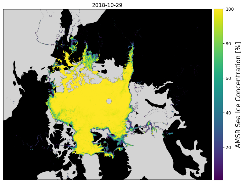

References¶

Spreen, G., Kaleschke, L., & Heygster, G. (2008). Sea ice remote sensing using AMSR‐E 89‐GHz channels. Journal of Geophysical Research: Oceans, 113(C2). 10.1029/2005jc003384