PS106 Broadband Solar Irradiance from the Ice Floe Camp

Dataset description¶

Title: Spatial and temporal variability of broadband solar irradiance during POLARSTERN cruise PS106/1 Ice Floe Camp (June 4th-16th 2017)

Authors Barrientos Velasco, Carola; Deneke, Hartwig; Macke, Andreas

Description The dataset is part of the expedition PS106/1 of the Research Vessel POLARSTERN to the Arctic Ocean in 2017. During the ice floe camp (drift period, June 4th-16th 2017) 15 pyranometer stations were deployed over the ice floe covering an area of about 1 km². Each station measured broadband solar irradiance and temperature at 1Hz resolution.

Relative humidity was also measured, however its use is not recommended due to technical problems of the sensors.

Each file contains horizontal level and cleanliness flags describing the status of the pyranometer dome per day. The criterion is as follows.

Cleanliness clean =1, drops =2, frozen =3, no observation = 4

Leveling leveled =1, partially leveled =2, unleveled =3, no observation =4

Year 2018

Institutes Tropos, Leipzig

DOI Barrientos Velasco et al. (2018)

License Creative Commons Attribution 4.0 International

Contents of this notebook¶

This notebook provides a minimal working example of reading and plotting broadband solar irradiance data from the POLARSTERN cruise PS106/1 Ice Floe Camp (June 4th-16th 2017). The data is visualized

a.) plotting the start positions of the measurement stations

b.) plotting the measured downward irradiance against time

for one day.

General information about this notebook¶

This notebook series has been initiated by the Data Management Project (INF) within the TR-172 “ArctiC Amplification: Climate Relevant Atmospheric and SurfaCe Processes, and Feedback Mechanisms” (AC)³ funded by the German Research Foundation (Deutsche Forschungsgemeinschaft, DFG)

Author(s) of this notebook:

Matthias Buschmann, Institute of Environmental Physics, University of Bremen, Germany, m_buschmann@iup.physik.uni-bremen.de
Jonas Hachmeister, Institute of Environmental Physics, University of Bremen, Germany, jonas_h@iup.physik.uni-bremen.de
Johannes Röttenbacher, Institute of Environmental Physics, University of Bremen, Germany, jroettenbacher@iup.physik.uni-bremen.de

GitHub repository: https://github.com/ac3-tr/ac3-book

This notebook is licensed under the Creative Commons Attribution 4.0 International

Import relevant modules¶

The following packages are needed for the execution of this notebook: matplotlib, numpy, cartopy, xarray

import cartopy.crs as ccrs
from cycler import cycler
import matplotlib.pyplot as plt
import numpy as np
import pangaeapy as pan
import xarray as xr

Pre-processing of the imported data¶

The data set consists of netCDF files, which can be downloaded using the pangaeapy module. For this example we only want the first file.

# Get the data using pangaeapy
import nest_asyncio
nest_asyncio.apply()

datafolder = '/media/jr/JR_SSD/tmp/pangaeapy_cache'  # adjust this to your local environment
ds = pan.PanDataSet(896710, enable_cache=True, cachedir=datafolder)
filenames = ds.download(indices=[0])

File pyrnet_ac3-pascal_2017-06-04_all.v2.nc already exists, skipping.

Read the downloaded NetCDF file¶

Let’s take a look at the netCDF file.

fname = filenames[0]
ds = xr.open_dataset(fname)
ds

If we look above, we notice that lat and lon aren’t actually coordinates but variables dependent on time. They track the drift of the individual stations. So we should correct that and can then also plot a simple map of the start positions of each station for the day of the data set. We also remove all nan values from the data set.

ds = ds.reset_coords(["lat", "lon"])
ds = ds.dropna('time')
ds

Let’s figure out the maximum extents of our data for our plot.

min_lat, max_lat, min_lon, max_lon = np.min(ds.lat), np.max(ds.lat), np.min(ds.lon), np.max(ds.lon)
print(f'Minimum Latitude: {min_lat.to_numpy():.4f}\n'
      f'Maximum Latitude: {max_lat.to_numpy():.4f}\n'
      f'Minimum Longitude: {min_lon.to_numpy():.4f}\n'
      f'Maximum Longitude: {max_lon.to_numpy():.4f}')

Minimum Latitude: 81.9286
Maximum Latitude: 81.9564
Minimum Longitude: 10.5393
Maximum Longitude: 10.7653

_, ax = plt.subplots(constrained_layout=True,
                     subplot_kw={'projection': ccrs.NorthPolarStereo()})
ax.set_prop_cycle(cycler(color=plt.get_cmap('tab20').colors))
ax.set_extent((10, 10.8, 81.9, 82))
ax.gridlines(draw_labels={"bottom": 'x', "right": "y"})
for station in ds.station:
    ds_sel = ds.sel(station=station).isel(time=0)
    ax.scatter(ds_sel.lon, ds_sel.lat, label=str(station.to_numpy()), transform=ccrs.PlateCarree())

ax.legend(ncols=2)
ax.set(
    title='Start Location of Radiation Stations - 2017-06-04',
)

[Text(0.5, 1.0, 'Start Location of Radiation Stations - 2017-06-04')]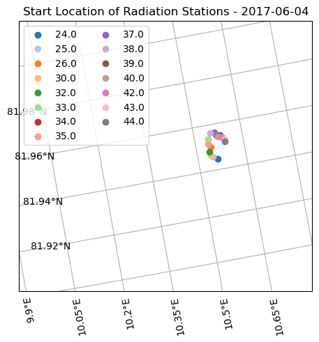

Plotting example¶

Overview plot¶

As an overview, we can plot the global horizontal irradiance against time for each station. Since there are 15 stations we split up the plot in 4 panels for better visibility of each line.

par = 'ghi'
ds[par]

tab20 = plt.get_cmap('tab20')
fig, axs = plt.subplot_mosaic(
    """
    AB
    CD
    """,
    constrained_layout=True,
    sharex=True, sharey=True,
)
ax = axs['A']
for i, station in enumerate(ds.station[0:4]):
    ds[par].sel(station=station).plot(x='time', ax=ax,
                                      label=str(station.to_numpy()),
                                      color=tab20(i))
ax.set(
    xlabel='',
    ylabel='Global horizontal\n irradiance (W$\\,$m$^{2}$)',
    title='',
)

ax = axs['B']
for i, station in enumerate(ds.station[4:8]):
    ds[par].sel(station=station).plot(x='time', ax=ax,
                                      label=str(station.to_numpy()),
                                      color=tab20(i+4))
ax.set(
    xlabel='',
    ylabel='',
    title='',
)

ax = axs['C']
for i, station in enumerate(ds.station[8:12]):
    ds[par].sel(station=station).plot(x='time', ax=ax,
                                      label=str(station.to_numpy()),
                                      color=tab20(i+8))
ax.set(
    xlabel='Time (UTC)',
    ylabel='Global horizontal\n irradiance (W$\\,$m$^{2}$)',
    title='',
)

ax = axs['D']
for i, station in enumerate(ds.station[12:]):
    ds[par].sel(station=station).plot(x='time', ax=ax,
                                      label=str(station.to_numpy()),
                                      color=tab20(i+12))
ax.set(
    xlabel='Time (UTC)',
    ylabel='',
    title='',
)

for name, ax in axs.items():
    ax.grid()
    ax.legend(title='Station')

fig.suptitle('2017-06-04')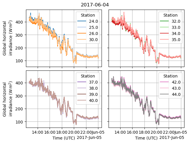

References¶

Barrientos Velasco, C., Deneke, H., & Macke, A. (2018). Spatial and temporal variability of broadband solar irradiance during POLARSTERN cruise PS106/1 Ice Floe Camp (June 4th-16th 2017). PANGAEA. 10.1594/PANGAEA.896710