Melt pond fraction from Sentinel-2

Dataset resources¶

The data of the operational sea ice concentration product can be downloaded via the link given below.

Authors: Niehaus, H. and Spreen, G.

Year: 2022

Institute: Institute of Environmental Physics, University of Bremen

URL: Niehaus & Spreen (2022)

Citeable Publication: Niehaus, H., Spreen, G., Birnbaum, G., Istomina, L., Jäkel, E., Linhardt, F., et al. (2023). Sea ice melt pond fraction derived from Sentinel-2 data: Along the MOSAiC drift and Arctic-wide. Geophysical Research Letters, 50, e2022GL102102. Niehaus et al. (2023)

General information about this notebook¶

This notebook series has been initiated by the Data Management Project (INF) within the TR-172 “ArctiC Amplification: Climate Relevant Atmospheric and SurfaCe Processes, and Feedback Mechanisms” (AC)³ funded by the German Research Foundation (Deutsche Forschungsgemeinschaft, DFG)

Author(s) of this notebook:

Hannah Niehaus, Institute of Environmental Physics, University of Bremen, Germany, niehaus@uni-bremen.de
Johannes Röttenbacher, Institute of Environmental Physics, University of Bremen, Germany, jroettenbacher@iup.physik.uni-bremen.de

GitHub repository: https://github.com/ac3-tr/ac3-book

This notebook is licensed under the Creative Commons Attribution 4.0 International

Reading example dataset¶

The data set consists of multiple netCDF files. We can access and download them using pangaeapy. For this example we are using a scene from the 19 July 2021.

import matplotlib.pyplot as plt
import numpy as np
import cartopy.crs as ccrs
import cartopy
from pangaeapy import PanDataSet
import xarray as xr

%matplotlib inline

# change this to your local data directory
cachedir = './data'
ds = PanDataSet(950885, enable_cache=True, cachedir=cachedir)
filename = ds.download(indices=[3])

File 20210719_T45XVK_s2_mpf.nc already exists, skipping.

data = xr.open_dataset(filename[0])
#print(data.variables['thickness'])
mpf = data['mpf']*100
x = data['x']
y = data['y']
date = data.date
zone = int(data.zone[:-1])

crs = ccrs.UTM(zone)
land110m = cartopy.feature.NaturalEarthFeature('physical', 'land', '110m', edgecolor='None', facecolor='k')
ocean110m = cartopy.feature.NaturalEarthFeature('physical', 'ocean', '110m', edgecolor='None', facecolor='lightgray')

fig = plt.figure(figsize=(15, 8))
ax = fig.add_subplot(111, projection=crs)
ax.set_title(f'{date[:4]}-{date[4:6]}-{date[6:]}')
# we could add these feature for larger maps or swaths close to the coast
# ax.add_feature(ocean110m)
# ax.add_feature(land110m)
cmap = plt.get_cmap('viridis')
cmap.set_under(color='white')
im = ax.imshow(mpf,
               extent=[np.nanmin(x),np.nanmax(x),np.nanmin(y),np.nanmax(y)],
               zorder=2,
               vmin=0.01,  # define something slightly greater than one to mimic closed sea ice
               cmap=cmap,
               )
gl = ax.gridlines(draw_labels=True, dms=False, x_inline=False, y_inline=False,linestyle = '--',color='black', transform=crs)
cb = fig.colorbar(im, ax=ax, fraction=0.024, pad=0.08)
cb.set_label('Melt pond fraction [%]', fontsize=15)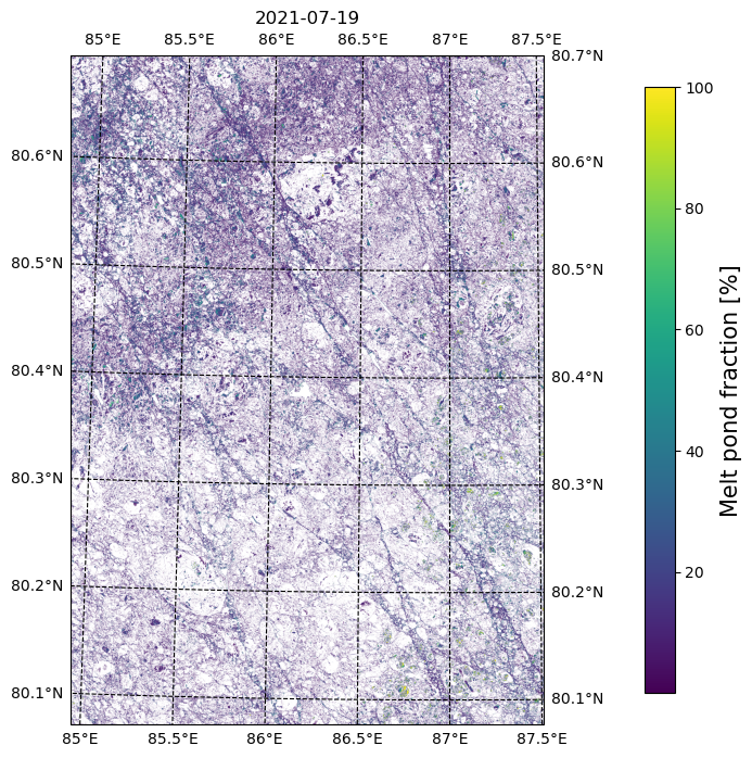

References¶

Niehaus, H., & Spreen, G. (2022). Melt pond fraction on Arctic sea-ice from Sentinel-2 satellite optical imagery (2017-2021). PANGAEA. 10.1594/PANGAEA.950885
Niehaus, H., Spreen, G., Birnbaum, G., Istomina, L., Jäkel, E., Linhardt, F., Neckel, N., Fuchs, N., Nicolaus, M., Sperzel, T., Tao, R., Webster, M., & Wright, N. (2023). Sea Ice Melt Pond Fraction Derived From Sentinel‐2 Data: Along the MOSAiC Drift and Arctic‐Wide. Geophysical Research Letters, 50(5). 10.1029/2022gl102102