Introduction to a cyclone cluster climatology dataset based on ERA5

Author of this notebook:

Lars Aue, Alfred Wegener Institute, Helmholtz Centre for Polar and Marine Research, lars.aue@awi.de

This notebook is licensed under the Creative Commons Attribution 4.0 International

Dataset description¶

Title: Climatology of serial cyclone clusters and solitary cyclones in the Arctic for 1979 to 2024

Author: Lars Aue

Year: 2026

Institute: Alfred Wegener Institute, Helmholtz Centre for Polar and Marine Research

DOI: Aue (2026)

License: Creative Commons Attribution 4.0 International

Abstract: This dataset provides a climatology of serial cyclone cluster and solitary cyclone events for the Arctic region including information on cyclone (cluster) occurrences and properties (event duration, cyclone intensity, cyclone cluster size). The dataset is derived from 6-hourly sea level pressure fields from the ERA5 reanalysis (Hersbach et al., 2020) by applying the Multi-Object Analysis of Atmospheric Phenomena (MOAAP) tracking tool (Prein et al., 2023) version V1.1.1 (https://github.com/AndreasPrein/MOAAP) and additional post-processing routines to separate the detected cyclone events into serial clusters and solitary cyclones. The separation is based on a maximum allowed time gap of 48 hours between consecutive cyclone passages. The dataset is available on the Equal-Area Scalable Earth (EASE) grid version 2.0 (Brodzik et al., 2012) with 25km² horizontal resolution and covers the years 1979 to 2024 with a daily temporal resolution. Hereby, days with a cyclone occurrence for at least one, 6-hourly timestep are considered as cyclone days.

Contents of this notebook¶

This notebook illustrates how to load the cyclone cluster dataset (which can be retrieved via zenodo) and create a simple climatology plot for solitary cyclones and serial cyclone clusters in the Arctic.

Import relevant modules¶

import xarray as xr
import matplotlib.pyplot as plt
import cartopy.crs as ccrs
import numpy as np

Load and pre-process data¶

You can download the data as a zip file from here: https://zenodo.org/records/18400261/files/CycloneClusterClimatology_ERA5_1979_2024.zip?download=1 Then unzip it on a folder and replace the data_path variable below with your complete path. The dataset is opened using xarray, afterward it is cut to the desired years and months.

### Set parameters ###
years = np.arange(2000,2010)
months = [12,1,2]

### Choose appropriate datasets based on years ###
#data_path = '/media/jr/JR_SSD/data/20260122_aue/'
# Change this to your path
data_path = '/path/to/netcdf_files/'

list_files = [data_path + 'CycloneClusterClimatology_ERA5_{}.nc'.format(y) for y in years]
data = xr.open_mfdataset(list_files)

### Cut to selected months ###    
data = data.sel(time=data.time.dt.month.isin([months]))

data

Exploration of dataset¶

The following section presents the variables contained in the dataset

The variable Cyclones_all contains a binary cyclone occurrence mask. “1” indicates that the grid-cell was situated within a cyclone for at least one, 6-hourly timestep of the current day, “0” indicates that no cyclone was present at that day. If the same cyclone is situated over a specific grid-cell for more than one day, multiple successive “1” entries are found.

data['Cyclones_all']

The variables CY_Objects_1st and CY_Clusters_1st contain a “1” whenever a specific solitary cyclone (or cyclone cluster) first reached a certain grid-cell. Thus, they can be used to count the number of occurrences of different cyclones (or cyclone clusters) at a grid-cell.

data['CY_Objects_1st']

data['CY_Clusters_1st']

The variables CY_Objects_dur and CY_Clusters_dur indicate how long the cyclone (or cyclone cluster) which first reached a grid-cell at that day remained at that specific grid-cell. The value is given in hours and based on the original, 6-hourly cyclone tracking output. If no new cyclone (cluster) reached the grid-cell, the value is “0”.

data['CY_Objects_dur']

data['CY_Clusters_dur']

The variables CY_Objects_intensity and CY_Clusters_intensity indicate the average intensity of the cyclone (or cyclone cluster) which first reached a grid-cell at that day. The intensity is defined as max. minus min. sea level pressure within the cyclone area and averaged over all timesteps, where the cyclone (cluster) was present at the specific grid-cell. If no new cyclone (cluster) reached the grid-cell, the value is “0”.

data['CY_Objects_intensity']

data['CY_Clusters_intensity']

The variable CY_Clusters_size contains the size of each cyclone cluster (number of clustered cyclones). A minimum threshold can be defined to mask all clusters below a certain size (example below). Solitary cyclones by definition always consist of only one cyclone, so there is no equivalent “size” variable for solitary cyclones.

data['CY_Clusters_size']

min_size=2
mask_min_size = 1 * (data['CY_Clusters_size']>=min_size)

data['CY_Clusters_1st'] = data['CY_Clusters_1st'] * mask_min_size
data['CY_Clusters_dur'] = data['CY_Clusters_dur'] * mask_min_size
data['CY_Clusters_size'] = data['CY_Clusters_size'] * mask_min_size

Plotting/Analysis example¶

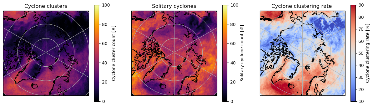
The following example demonstrates how to plot the number of solitary cyclone and cyclone cluster cases in the Arctic, as well as the overall clustering rate of cyclones (share of all cyclones, which occur within clusters).

### Calculate total number of cyclone (cluster) occurrences  ###
N_clusters = data['CY_Clusters_1st'].astype('float').sum(dim='time')
N_solitary = data['CY_Objects_1st'].astype('float').sum(dim='time')

N_clustered_cyclones = data['CY_Clusters_size'].astype('float').sum(dim='time')
N_all_cyclones = N_solitary + N_clustered_cyclones

### Choose domain for plotting ###
domain = [0,359.9,60,90]  # lon_min, lon_max, lat_min, lat_max

### Choose appropriate minima and maxima for the colorscale ###
vmin = 0
vmax = 100

vmin_rate = 10
vmax_rate = 90

### Create a figure with 3 subplots: Absolute number of cyclone clusters, absolute number of solitary cyclones, clustering rate (number of clustered cyclones divided by number of all cyclones) ###
plt.figure(figsize=(15,4))

ax0 = plt.subplot(1, 3, 1, projection=ccrs.NorthPolarStereo())                            
ax0.gridlines()
ax0.coastlines(resolution='50m')
ax0.set_extent(domain,
              crs=ccrs.PlateCarree()
              )

ax0.set_title('Cyclone clusters')

h0 = ax0.pcolormesh(data.lon,data.lat,N_clusters,
              transform=ccrs.PlateCarree(),
              cmap='inferno',
              vmin=vmin,
              vmax=vmax
              )

plt.colorbar(h0,label='Cyclone cluster count [#]')

ax1 = plt.subplot(1, 3, 2, projection=ccrs.NorthPolarStereo())                            
ax1.gridlines()
ax1.coastlines(resolution='50m')
ax1.set_extent(domain,
              crs=ccrs.PlateCarree()
              )

ax1.set_title('Solitary cyclones')

h1 = ax1.pcolormesh(data.lon,data.lat,N_solitary,
              transform=ccrs.PlateCarree(),
              cmap='inferno',
              vmin=vmin,
              vmax=vmax
              )

plt.colorbar(h1,label='Solitary cyclone count [#]')

ax2 = plt.subplot(1, 3, 3, projection=ccrs.NorthPolarStereo())                            
ax2.gridlines()
ax2.coastlines(resolution='50m')
ax2.set_extent(domain,
              crs=ccrs.PlateCarree()
              )

ax2.set_title('Cyclone clustering rate ')

h2 = ax2.pcolormesh(data.lon,data.lat,100 * np.round(N_clustered_cyclones/N_all_cyclones,2),
              transform=ccrs.PlateCarree(),
              cmap='coolwarm',
              vmin=vmin_rate,
              vmax=vmax_rate
              )

plt.colorbar(h2,label='Cyclone clustering rate [%]')

/sw/spack-levante/mambaforge-22.9.0-2-Linux-x86_64-kptncg/lib/python3.10/site-packages/dask/core.py:119: RuntimeWarning: invalid value encountered in divide
  return func(*(_execute_task(a, cache) for a in args))

References¶

Aue, L. (2026). Climatology of serial cyclone clusters and solitary cyclones in the Arctic for 1979 to 2024. Zenodo. 10.5281/ZENODO.18400261